Checkerboard calibration: Bouguet's example 1 in KIPES
Jean-Yves Bouguet's classic 20 checkerboard photos, calibrated step by step in KIPES - and KIPES's camera parameters next to the ones Bouguet published, with what differs and why.
The dataset: Bouguet's toolbox documentation with the 25 photos, one zip of 22.7 MB
The dataset
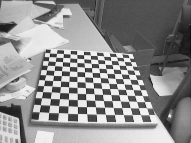
Jean-Yves Bouguet's camera calibration toolbox comes with a first calibration example that has taught camera calibration for more than twenty years: 20 photos, 640 × 480 pixels, of a checkerboard with 14 × 13 squares of 30 mm. Caltech publishes the toolbox's documentation with the photos at CaltechDATA under CC BY, and the documentation prints Bouguet's results for them. They are the yardstick for KIPES on this page.
Download calib_doc.zip (22.7 MB) from the dataset's page and unpack it. In its folder htmls, unpack calib_example.zip: Image1.tif to Image20.tif. Five more photos, Image21.tif to Image25.tif, lie directly in htmls.
1. Create a space and a subspace
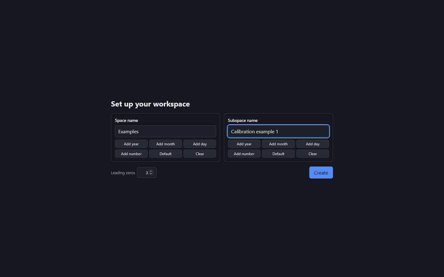
On the first start, KIPES opens Set up your workspace. Type a space name and a subspace name (here Examples and Calibration example 1) and press Create.
2. Import the photos
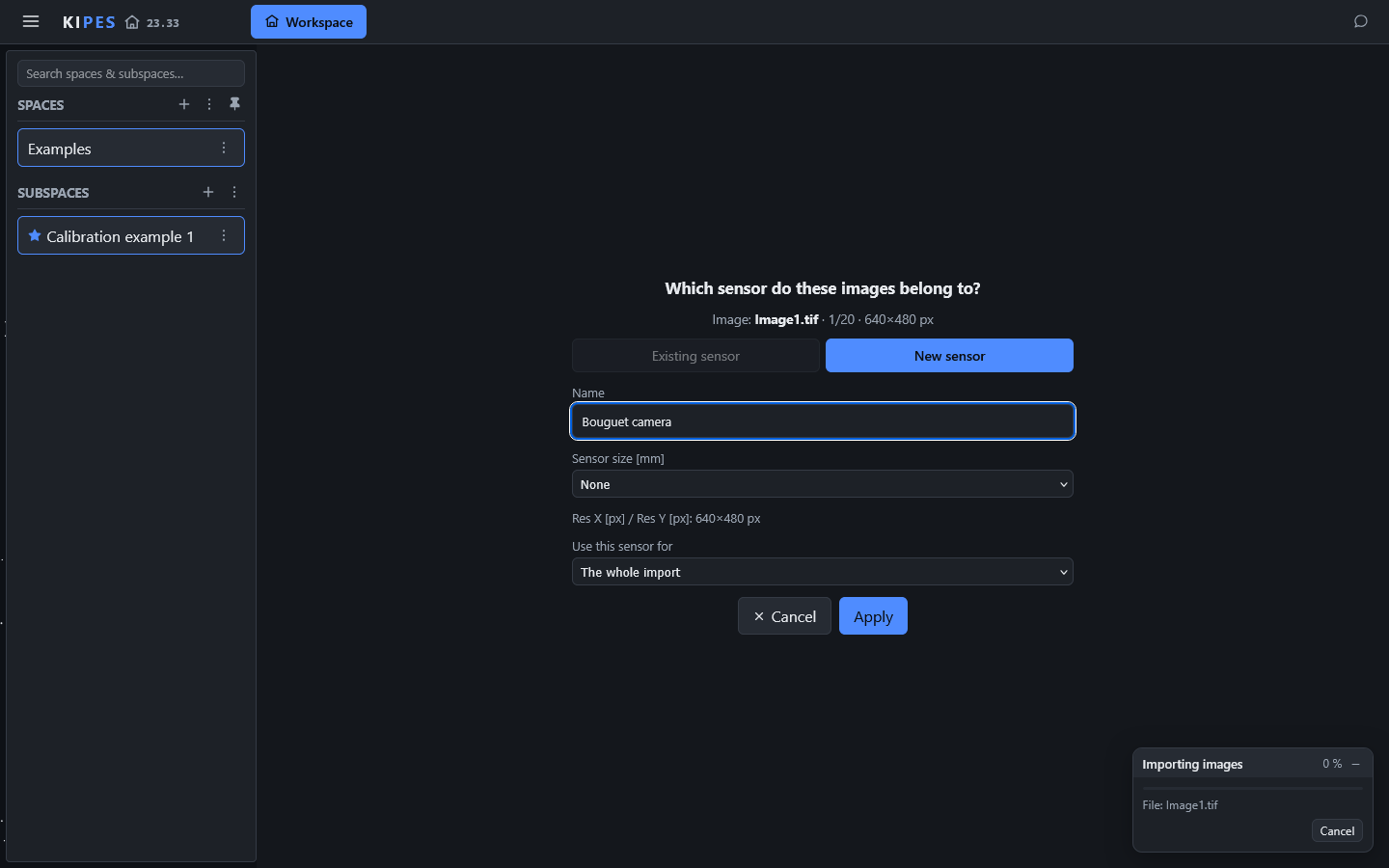
On the Workspace tab, the import button of the Images card opens the file dialog: select Image1.tif to Image20.tif. KIPES asks once for the camera. Give it a name (here Bouguet camera), leave Sensor size at None - the dataset names no sensor, and KIPES then works in pixels - keep The whole import and press Apply.
3. Detect the corners
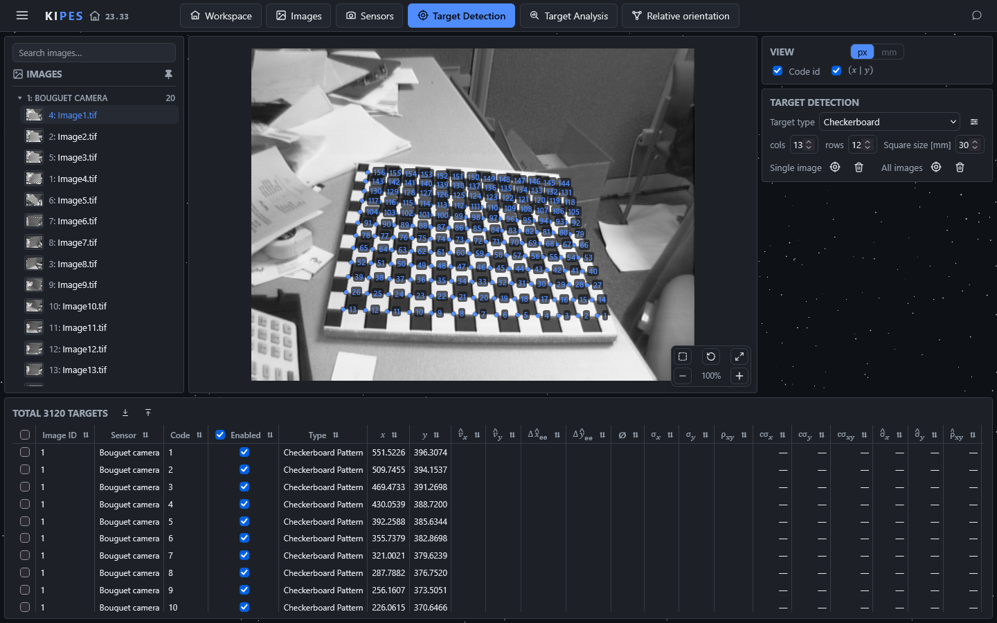
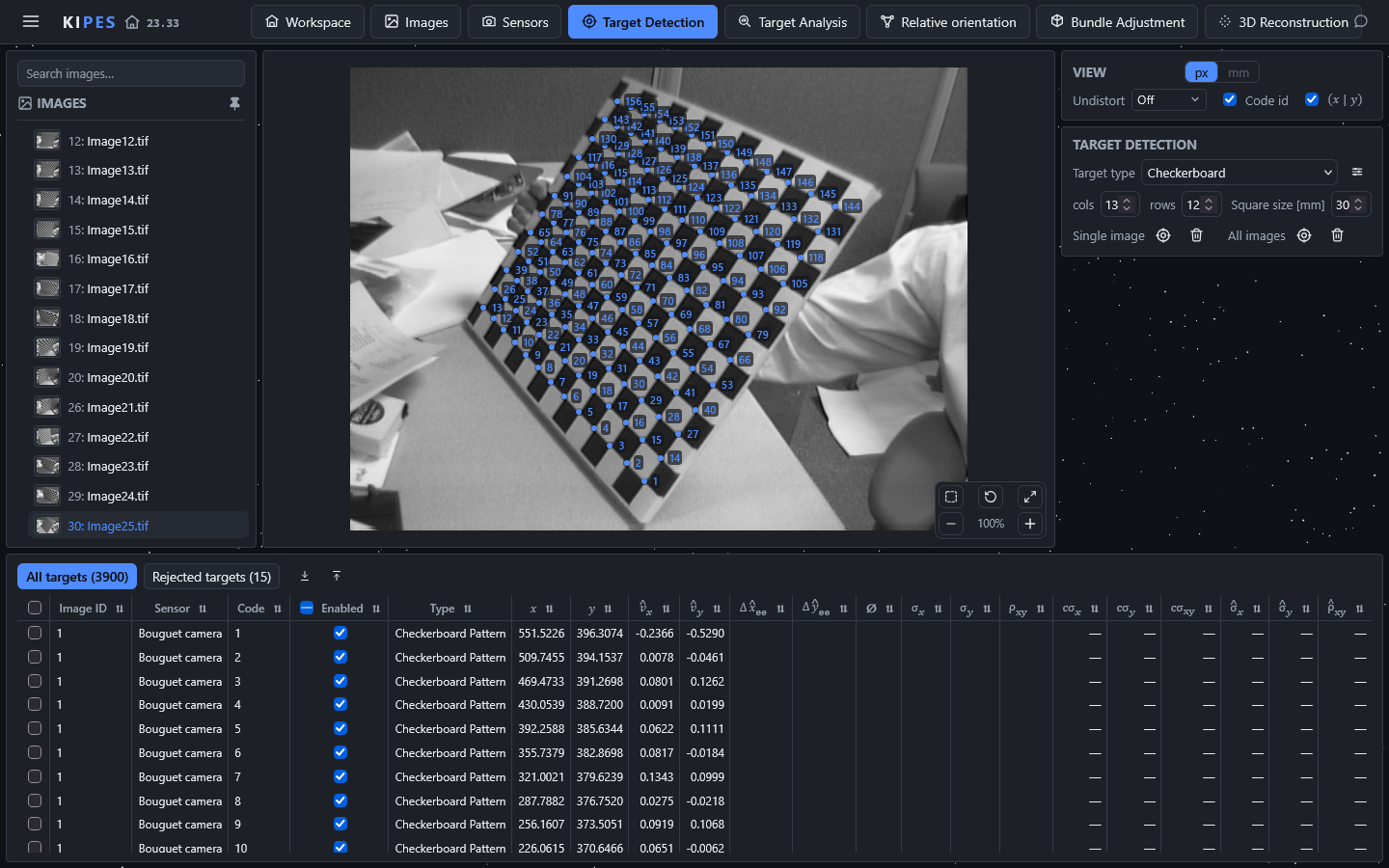
Open Target Detection and choose the target type Checkerboard. KIPES counts the board's inner corners: cols 13 and rows 12 for 14 × 13 squares. Set Square size [mm] to 30 and detect on All images. KIPES finds all 156 corners in each of the 20 photos, 3 120 in all, and numbers them the same way in every photo.
4. Choose Bouguet's camera model
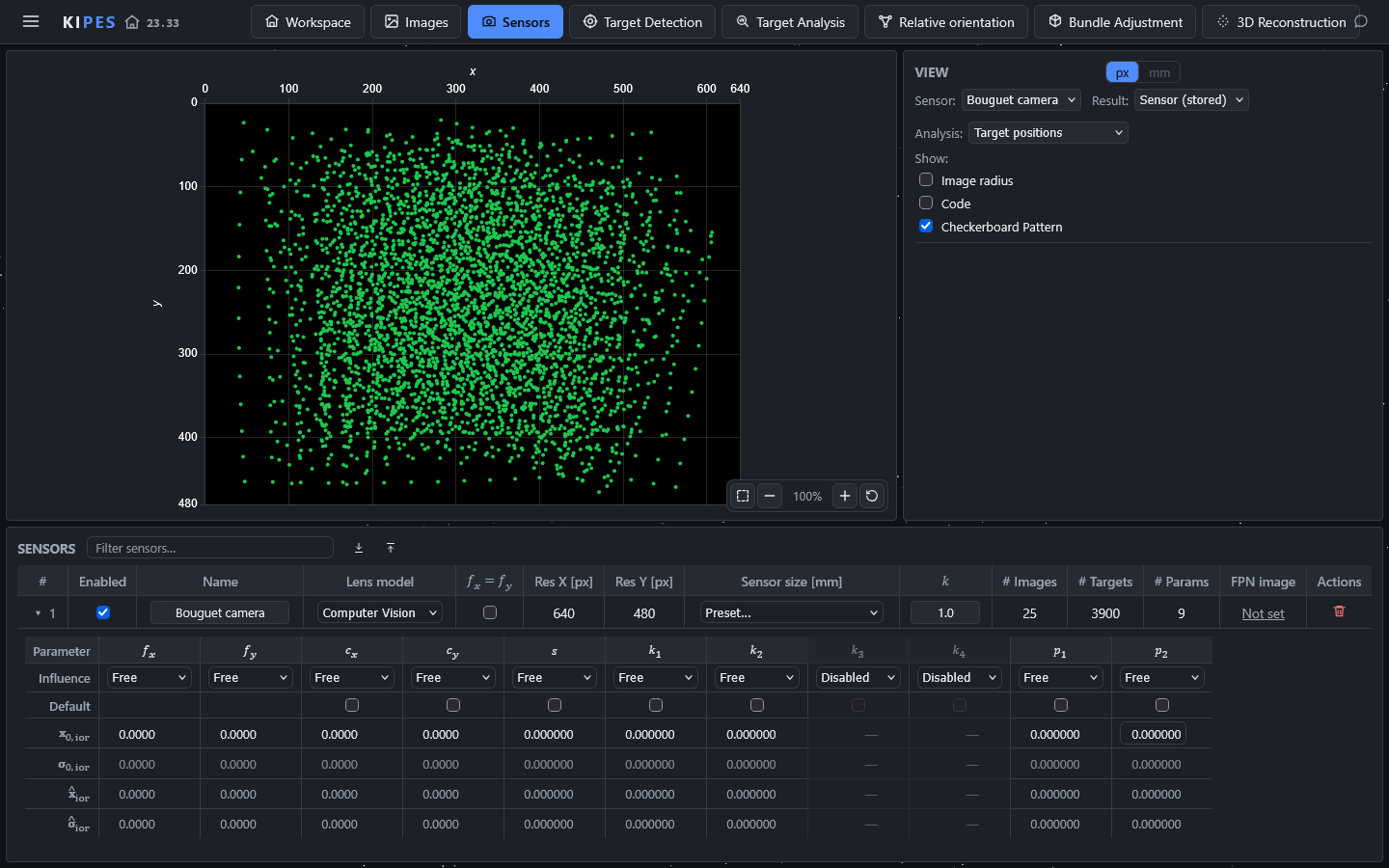
On the Sensors tab, set the Lens model to Computer Vision. Its parameters are Bouguet's: the focal lengths fx and fy, the principal point, the skew s, the radial distortion k1, k2 and k3, and the tangential distortion p1 and p2. Bouguet's main result estimates two focal lengths and leaves out the skew and k3, so:
- untick fx = fy,
- set k3 to Disabled,
- leave s at Fixed (0) and the rest at Free.
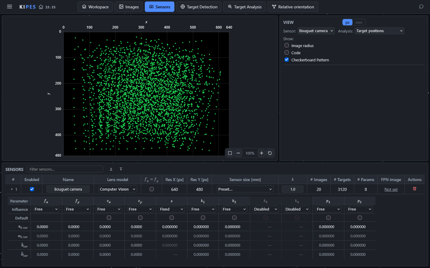
The plot shows where the corners lie on the sensor. The 20 photos cover the image out to its corners, which is what a calibration of the distortion needs.
5. Orient the cameras
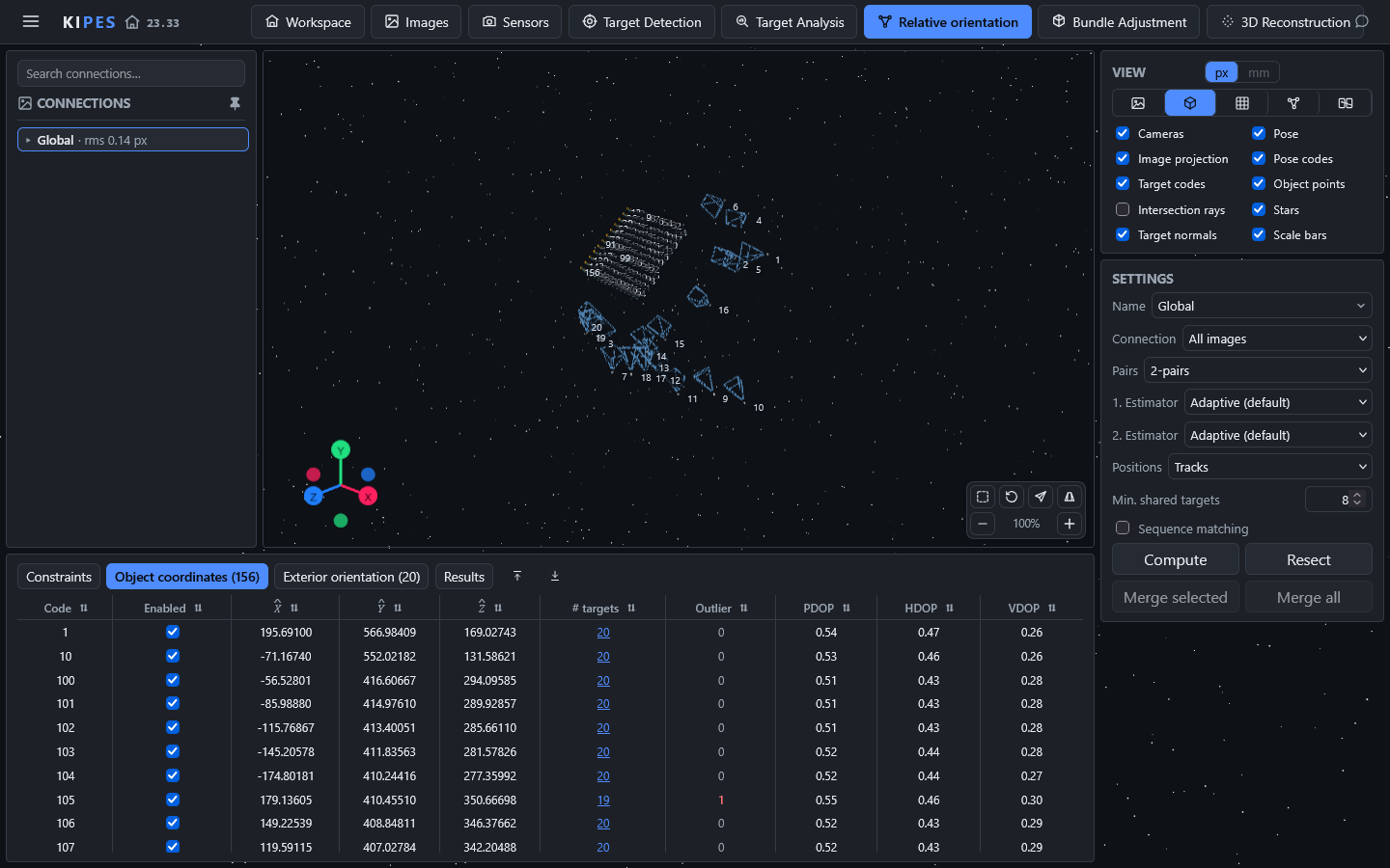
Open Relative orientation and press Compute with the settings as they are. The 20 cameras take their places around the board, with an rms of 0.14 px.
6. Calibrate the camera in the bundle adjustment
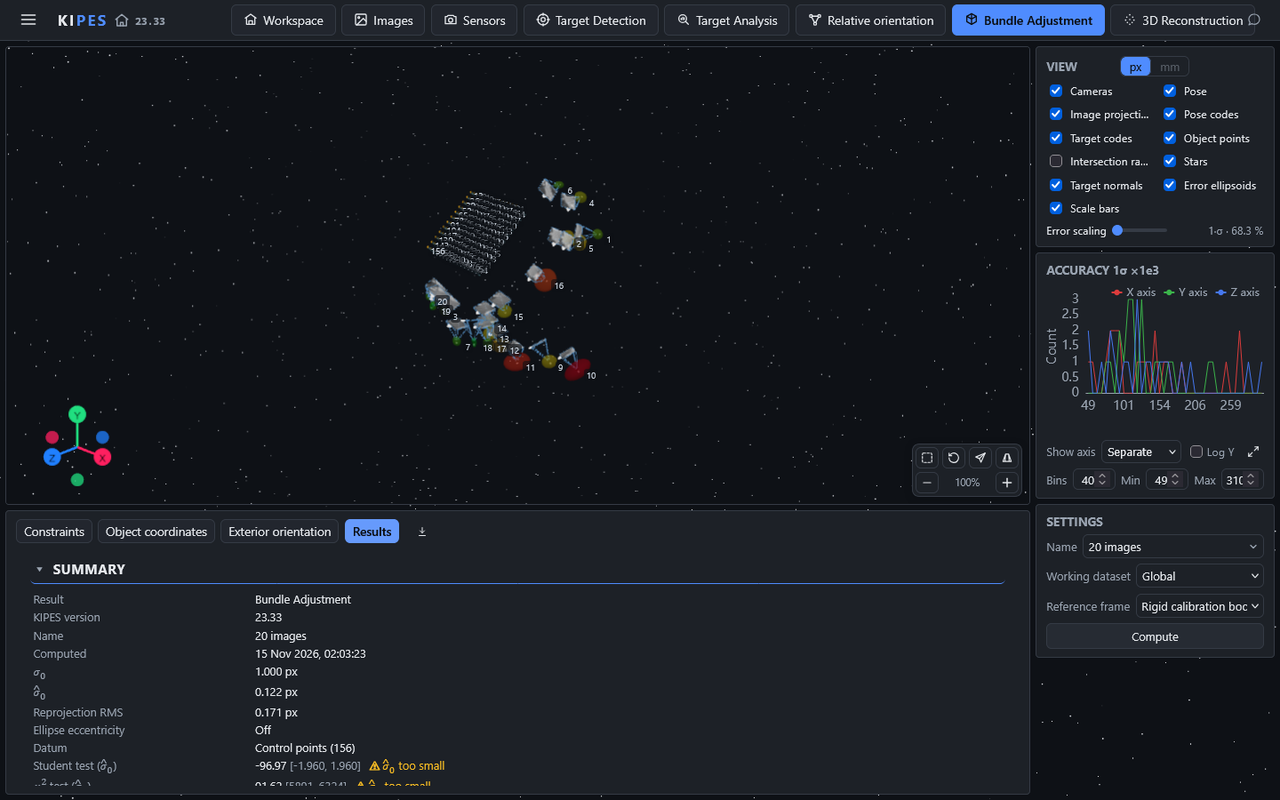
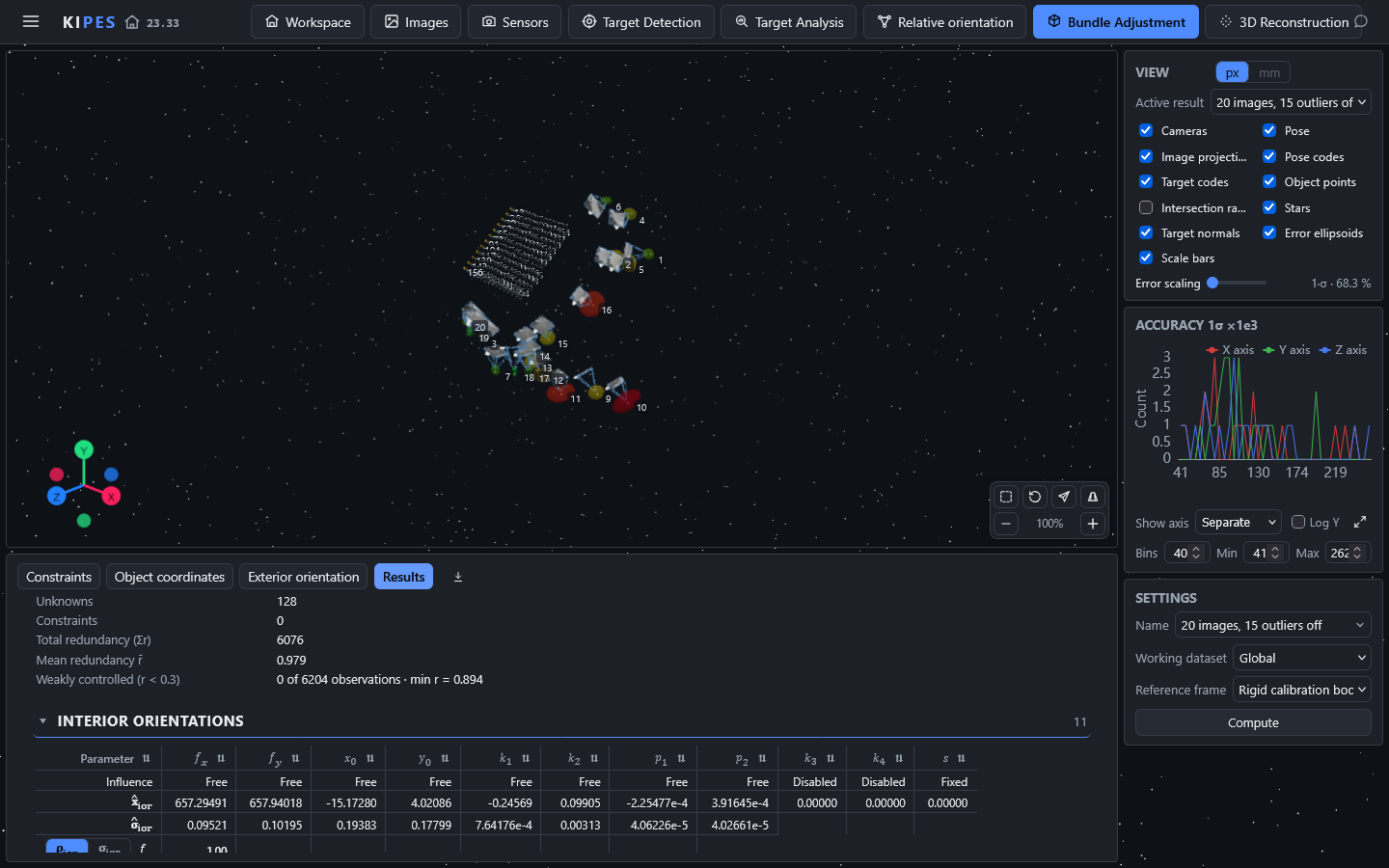
Open Bundle Adjustment, give the result a name and press Compute. The board is the reference: KIPES builds its 156 corners from the rows, the columns and the square size and holds them fixed - the summary says Datum: Control points (156). As in Bouguet's toolbox, the camera and the 20 positions of the board are computed together.
The corners fit with σ̂0 = 0.122 px. The three tests of σ̂0 warn that it is too small: a corner found in a photo carries no accuracy of its own, so KIPES weights it with 1 px, and the adjustment finds the corners eight times better than that. The warnings say exactly this; they do not mark a problem of the calibration.
7. Take out the outliers
KIPES tests every corner against all the others. In the Results, type flagged into the filter of the outlier test under Image coordinates: 15 corners are marked, one in Image4.tif, four in Image5.tif and ten in Image16.tif (3 more the orientation had already set aside). Two of them, corners 1 and 79 of Image5.tif, lie more than 3 px from where the adjustment puts them. Target Analysis shows why: at the edge of the board, seen at a steep angle, corner 1 was found above the crossing of the squares.
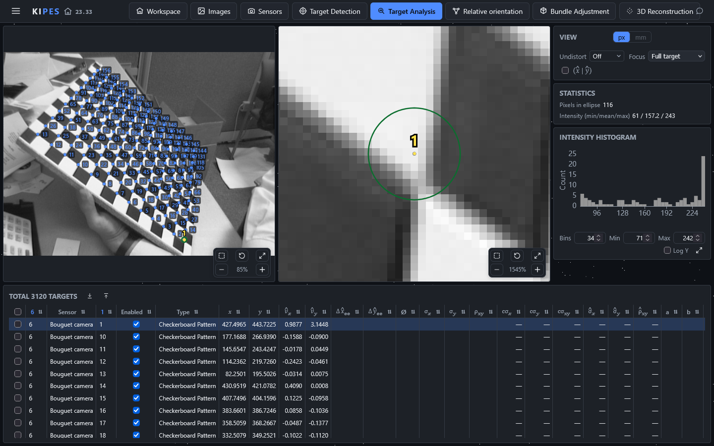
Untick Enabled for the 15 corners in Target Analysis and press Compute on Bundle Adjustment again. The remaining 3 102 corners fit with σ̂0 = 0.104 px - a tenth of a pixel per coordinate.
8. The calibration
Results, Interior orientations lists the parameters with their standard deviations. KIPES shows the principal point as x0 and y0, measured from the centre of the image.
9. Five more photos, and the skew
Bouguet then adds Image21.tif to Image25.tif and finally estimates the skew. In KIPES:
- Import the five photos and choose the existing sensor, Bouguet camera.
- In Target Detection, select each new photo and detect on Single image. All images would detect all 25 anew and switch the 15 outliers back on.
- Compute the Relative orientation again (Overwrite), then the Bundle Adjustment: 25 photos, σ̂0 = 0.104 px.
- On the Sensors tab, set s to Free and compute the bundle adjustment once more.
KIPES next to Bouguet
Two things have to be put on the same footing before the numbers can be compared:
- Standard deviations: KIPES gives one standard deviation; Bouguet's printout gives about three ("The numerical errors are approximately three times the standard deviations"). His values are divided by three here.
- The principal point: KIPES shows it from the centre of the image and counts the centre of the top-left pixel as (1, 1); Bouguet counts that centre as (0, 0). So Bouguet's cx is 319 + x0 and his cy is 239 + y0: KIPES's x0 = −15.173 px becomes cx = 303.827 px.
| Parameter | KIPES | Bouguet | KIPES − Bouguet | in σ |
|---|---|---|---|---|
| fx [px] | 657.295 ± 0.095 | 657.463 ± 0.106 | −0.168 | −1.2 |
| fy [px] | 657.940 ± 0.102 | 657.947 ± 0.113 | −0.007 | 0.0 |
| cx [px] | 303.827 ± 0.194 | 303.137 ± 0.216 | +0.691 | +2.4 |
| cy [px] | 243.021 ± 0.178 | 242.569 ± 0.197 | +0.452 | +1.7 |
| k1 | −0.24569 ± 0.00076 | −0.25403 ± 0.00083 | +0.00834 | +7.4 |
| k2 | 0.0991 ± 0.0031 | 0.1214 ± 0.0033 | −0.0224 | −4.9 |
| p1 | −0.00023 ± 0.00004 | −0.00021 ± 0.00004 | −0.00002 | −0.3 |
| p2 | 0.00039 ± 0.00004 | 0.00002 ± 0.00004 | +0.00037 | +6.3 |
| fit per coordinate [px] | 0.104 | 0.117 (x), 0.115 (y) |
The last column divides the difference by its own standard deviation, the two programs' standard deviations combined.
| Parameter | KIPES | Bouguet | KIPES, skew | Bouguet, skew |
|---|---|---|---|---|
| fx [px] | 657.131 ± 0.085 | 657.296 ± 0.095 | 657.137 ± 0.085 | 657.303 ± 0.095 |
| fy [px] | 657.760 ± 0.087 | 657.746 ± 0.097 | 657.759 ± 0.087 | 657.744 ± 0.096 |
| cx [px] | 303.712 ± 0.173 | 302.984 ± 0.193 | 303.520 ± 0.177 | 302.717 ± 0.197 |
| cy [px] | 242.847 ± 0.166 | 242.478 ± 0.185 | 242.763 ± 0.167 | 242.334 ± 0.186 |
| pixel axes [°] | 90 (held) | 90 (held) | 89.983 ± 0.003 | 89.976 ± 0.004 |
| k1 | −0.24495 ± 0.00071 | −0.25340 ± 0.00077 | −0.24496 ± 0.00071 | −0.25349 ± 0.00077 |
| k2 | 0.0966 ± 0.0030 | 0.1188 ± 0.0032 | 0.0962 ± 0.0030 | 0.1187 ± 0.0031 |
| p1 | −0.00027 ± 0.00004 | −0.00027 ± 0.00004 | −0.00028 ± 0.00004 | −0.00028 ± 0.00004 |
| p2 | 0.00041 ± 0.00004 | 0.00002 ± 0.00004 | 0.00043 ± 0.00004 | 0.00005 ± 0.00004 |
| fit per coordinate [px] | 0.104 | 0.118 (x), 0.116 (y) | 0.104 | 0.117 (x), 0.116 (y) |
What differs, and why
The camera model, the photos and the kind of computation are the same. The corners are not: each program measures them itself. Bouguet clicked the four outer corners of the board in every photo, helped his corner finder with a guess of the distortion where it missed the corners otherwise, and chose the size of its search window photo by photo. KIPES finds and numbers the corners on its own. Everything in the tables follows from where the corners lie.
- The focal lengths agree to 0.17 px, or 0.03 %, within about one standard deviation.
- The fit: KIPES's corners fit the model with 0.104 px per coordinate, Bouguet's with 0.117 px in x and 0.115 px in y.
- k1 and k2 differ by 7 and 5 standard deviations - and still describe the same lens. KIPES reports why: k1 and k2 are correlated with −0.94, so a smaller k1 together with a smaller k2 bends the image in nearly the same way. Worked out with the model's formula for the radial distortion, both pairs move a point 400 px from the centre of the image inwards by 30.94 px, and nowhere in the image do the two differ by more than 0.23 px (310 px from the centre, where the distortion is 15.4 px).
- The principal point lies 0.7 px further right and 0.45 px lower in KIPES, and p2 differs too. The two belong together: KIPES reports x0 and p2 correlated with 0.62 (and y0 and p1 with 0.40) - a shift of the principal point and a tangential term can partly stand in for each other.
- Standard deviations tell how well the corners fit the model, not how the corners were measured: two careful measurements of the same corners can differ by more than the standard deviations suggest. Bouguet's own numbers show it. When he only measured the corners again with other window sizes, his fy moved by 0.18 px and his k2 by 0.006 - one and a half to two of his standard deviations.
- The outliers: KIPES marks corners in
Image4.tif,Image5.tifandImage16.tif. Bouguet, too, measures the corners of several photos again -Image5.tifamong them, with a window of its own - and leavesImage16.tifout in one of his variants. Corner 118 is marked in three photos at once, and in more once the first 15 are out: perhaps a corner of the board itself that does not lie quite where a perfect board would have it. Both programs take the board as perfect. - The skew: both programs find it different from zero by the statistics, and both negligible. The pixel axes stand at 89.983° in KIPES and at 89.976° in Bouguet's result; KIPES's s of 0.19 px moves a point at the top or bottom edge of the image by 0.07 px.